

By CrowdSent Blog Team
An automated market maker, or AMM, is a set of rules that prices exchanges against a pool of assets. In a blockchain implementation, smart contracts apply those rules and update the pool when a trade executes. Understanding an AMM starts with its inventory, pricing rule and fee treatment.
A pool can have a large dollar value while offering limited liquidity at a particular price. Its token balances can also change without a liquidity provider adding or removing funds. These are consequences of how the mechanism works, and they matter when interpreting decentralized-market data.
This guide uses a simplified constant-product pool to make those changes visible. The numbers are hypothetical, fees are initially excluded, and the example is an explanation of market structure rather than a recommendation to trade or provide liquidity.
What does an automated market maker actually automate?
The AMM automates the relationship between an incoming amount, an outgoing amount and the pool’s resulting state. A trader supplies one asset and receives another under a rule enforced by code. Liquidity providers supply the inventory against which those exchanges occur.
Consider three separate questions: what assets are in the pool, how the rule converts one into another, and who has a claim on what remains. Calling all three “liquidity” hides useful distinctions. The pool holds assets, the pricing rule determines exchanges, and the ownership mechanism assigns claims.
For example, Uniswap’s v2 swap documentation describes exchanges governed by a constant-product rule. This is a specific protocol design. The AMM category is broader, so an explanation of v2 should not be treated as a specification for every decentralized exchange.
Smart contracts supply the execution framework. The broader relationship between a network and applications built on it is covered in CrowdSent’s introduction to Ethereum and app activity.
How the constant-product rule changes reserves
In the simplest two-asset model, call the reserves x and y. The rule is x multiplied by y equals k. Ignoring fees and changes in supplied liquidity, k stays constant through a trade.
Suppose a pool contains 100 units of token A and 10,000 units of token B. Its product is 1,000,000. The reserve ratio is 100 B per A. That ratio describes the marginal price in this idealized model: the rate approached by a very small exchange before fees.
A finite trade moves the pool along its curve. The price therefore changes through the exchange. Multiplying the starting reserve ratio by the whole trade amount would skip the inventory change that the AMM is designed to capture.
A worked exchange with all assumptions visible
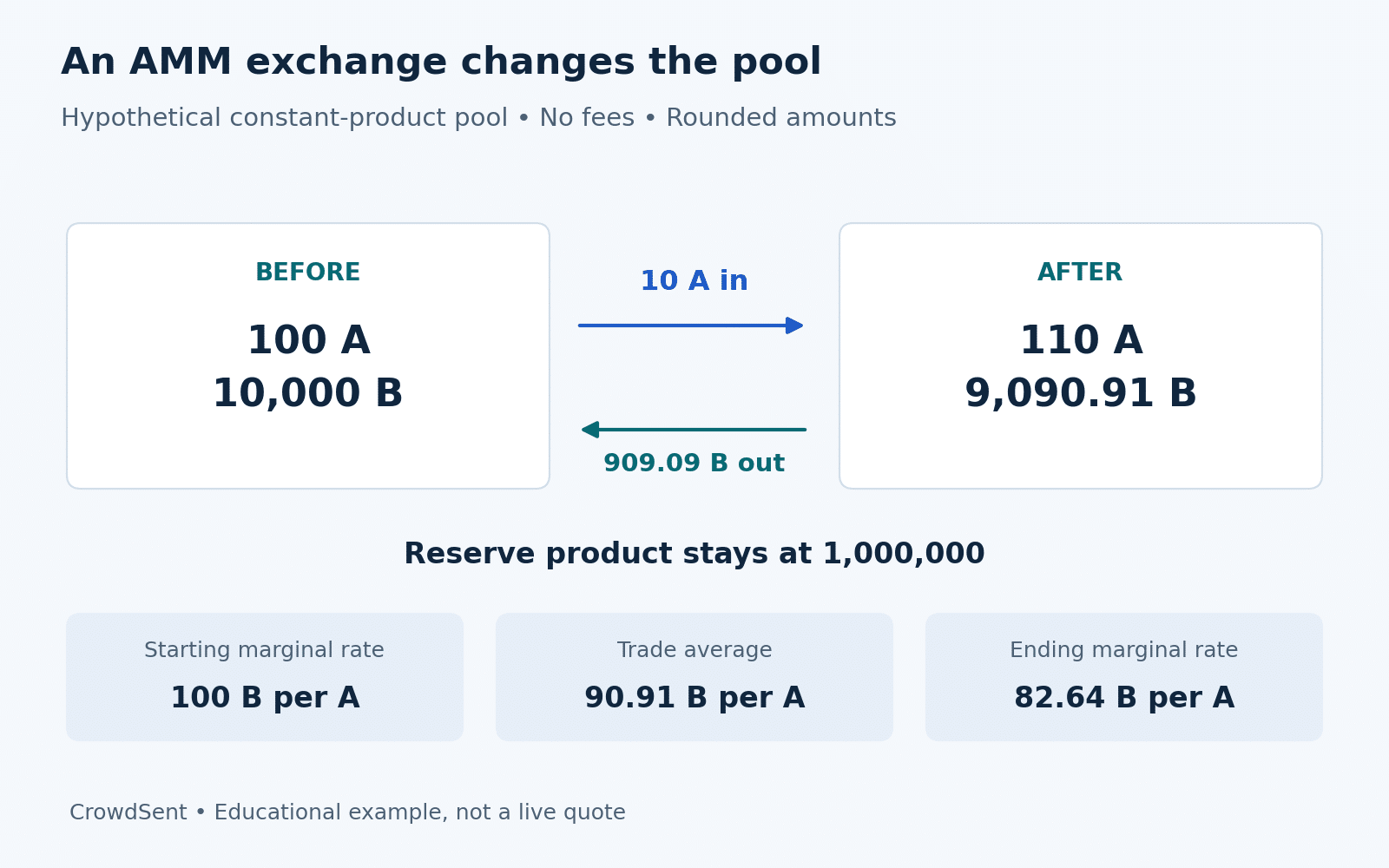
Imagine a trader adds 10 A to this pool. With no fee, the new A reserve is 110. To preserve the product, the B reserve becomes 1,000,000 divided by 110, or about 9,090.91 B.
The trader receives the difference between the old and new B reserves: 10,000 minus 9,090.91, or approximately 909.09 B. Dividing by the 10 A input gives an average execution rate of about 90.91 B per A.
After the exchange, the marginal reserve ratio is approximately 9,090.91 divided by 110, or 82.64 B per A. Three numbers now describe three different things: 100 was the starting marginal rate, 90.91 was the average rate for this exchange, and 82.64 is the ending marginal rate.
The example does not model a changing external market, other transactions, transaction costs or token-specific transfer behavior. It isolates the consequence of changing the reserves. Adding those omitted details requires a more complete model rather than a different interpretation of the same three numbers.
Why the size and shape of liquidity both matter
Now increase both starting reserves tenfold: 1,000 A and 100,000 B. The starting ratio remains 100 B per A. The same 10 A input produces approximately 990.10 B under the fee-free constant-product rule, for an average rate near 99.01 B per A.
The larger pool absorbs this particular exchange with less movement along the curve. The comparison is meaningful because the token pair, model, starting ratio and trade size were held constant. Comparing two headline pool values without those controls can be misleading.
Liquidity also has a distribution. Some designs spread it over a wide set of possible prices; others concentrate it in selected intervals. The amount relevant to an exchange depends on where that exchange travels. CrowdSent’s explanation of liquidity versus volume provides the complementary distinction between available capacity and activity already recorded.
How arbitrage connects the pool to other markets
The simple rule does not independently discover what an asset should be worth elsewhere. If another market changes while the pool remains unchanged, a difference can open between their exchange rates. Trading across that difference can move the pool’s reserve ratio toward the external market.
That adjustment has limits. Fees, transaction costs, delays and access to inventory affect whether a difference can be acted on. A pool price can temporarily diverge, particularly where trading is expensive or liquidity is thin.
The important accounting result is that reserve composition responds to trading. Someone with a constant percentage claim on the pool may end up exposed to fewer units of one asset and more of the other. A stable ownership percentage does not imply stable underlying quantities.
Uniswap’s v2 pool documentation connects initial reserve ratios, arbitrage and pool shares. Its protocol-specific description is useful evidence for this model, rather than a promise that all pools remain aligned at all times.
Where fees enter the explanation
A swap fee changes how much of the incoming amount contributes to the pricing calculation. Fee allocation also matters: some amounts may accrue to liquidity providers, while a protocol can have separate rules for its share.
For a purely hypothetical 0.30% input fee on the 10 A exchange, 9.97 A would enter the common fee-adjusted quote formula. The calculated output would be about 906.61 B. If the full 10 A remains in the pool and the fee stays with providers, the final reserve product grows instead of remaining exactly at its fee-free starting value.
This assumption should be stated explicitly. A fee percentage is not a universal AMM setting, and a pool’s total fees are not automatically an individual provider’s earnings. The relevant ownership share, active range and protocol deductions all require their own accounting.
Network transaction charges are another category. They should not be merged with a pool’s trading fee. CrowdSent’s guide to Ethereum gas fees explains that separate network cost.
How concentrated liquidity changes the picture
In Uniswap v3 and v4, liquidity can be allocated to selected price ranges. A position participates while the price is within its range. Once the price moves outside it, that position becomes inactive and stops earning swap fees until it is active again.
The official concentrated-liquidity documentation explains these boundaries. Their research implication is straightforward: total deposited value cannot reveal how much liquidity is active around the current price.
Imagine two pools each reported at a hypothetical $1 million. One has much of its liquidity near the current exchange rate; the other has most positions far away. Equal total value does not establish equal capacity for a nearby exchange. A meaningful comparison needs the range distribution as well as the total.
Why protocol version belongs in every AMM explanation
An AMM label is too broad to identify all applicable rules. The protocol, version, asset pair, fee configuration and any custom behavior help define the actual system being measured.
For example, Uniswap v4 hooks can add custom logic around pool actions. They are optional and pool-specific. Consequently, a familiar protocol name alone does not establish identical behavior across every pool associated with it.
A useful research note records the exact pool or position, the observation time and the assumptions behind any calculation. It separates a simplified model from an observed transaction. This makes an explanation reproducible without pretending that a small example captures all execution or smart-contract risks.
Frequently asked questions about automated market makers
1. Does an AMM need another trader at the same moment?
A funded pool supplies the inventory for an exchange, so an opposing trader does not need to submit a matching order simultaneously. Execution still depends on available liquidity and the contract’s rules. A pool with unsuitable assets or insufficient usable liquidity cannot satisfy every requested exchange.
2. Is the reserve ratio the price for my entire trade?
In the simplified constant-product model, it is the marginal rate before fees. A finite exchange changes reserves, so its average rate differs. The starting ratio, average exchange rate and ending ratio should be labeled separately whenever an example presents all three.
3. Does k stay constant forever?
No. Constant product describes a particular pricing constraint under stated assumptions. Fees retained in the pool and additions or removals of supplied liquidity can change the reserve product. Comparing k across dates without checking those events gives an incomplete account of what happened.
4. Does a larger pool always offer a better exchange rate?
For otherwise identical constant-product pools at the same starting price, larger reserves reduce the price movement from the same trade. Across different designs, however, range placement, fees, token behavior and available routes also matter. Headline size alone does not settle the comparison.
5. Who sets a new pool’s starting price?
In a basic two-reserve design, the initial quantities establish the starting ratio. That ratio can differ from other markets and invite arbitrage. Establishing an initial pool therefore does not certify a fair market valuation or guarantee that the ratio will persist.
6. Can an AMM work without an external price feed?
A basic constant-product swap can be calculated from pool reserves and its rule. External trading helps connect its ratio with other markets. Some AMM designs use additional information, so the presence or absence of external inputs must be checked for the specific implementation.
7. Are all liquidity providers earning fees simultaneously?
That depends on the model. In concentrated-liquidity systems, a position outside the current price range is inactive and does not earn swap fees during that interval. Pool-wide volume or fee totals therefore cannot be assigned equally to every position.
8. Are AMMs only available on Ethereum?
No. AMM mechanisms can be implemented on different networks. A network name does not specify the pool’s mathematics, permissions or accounting. Comparisons should identify both the chain and the actual protocol implementation rather than transferring assumptions from one deployment to another.
9. Does automation remove financial or technical risk?
Automation makes the stated rules executable. It does not eliminate asset-price changes, adverse changes in reserve composition, implementation errors or dependencies on other contracts. Understanding a rule is one part of research, and should not be read as evidence that a pool is safe.
10. Which observation best explains an AMM exchange?
A before-and-after record of reserves, inputs, outputs and fees is a useful starting point. For concentrated liquidity, include the relevant range and active liquidity. A headline dollar value or a screenshot of the starting price leaves important parts of the exchange unexplained.
Conclusion: follow the inventory through the rule
The clearest way to understand an automated market maker is to follow an exchange from starting reserves to ending reserves. That reveals the average rate, the changed composition and the assumptions required for the calculation. Protocol version, fees and liquidity distribution then explain where the simple model needs extending.
Keep this article as an educational reference when examining claims about decentralized-market liquidity.
Source documentation checked 11 October 2026. Educational explanation from the CrowdSent Blog Team. Numerical examples are hypothetical unless explicitly identified otherwise. This article does not provide investment recommendations.