

By CrowdSent Blog Team
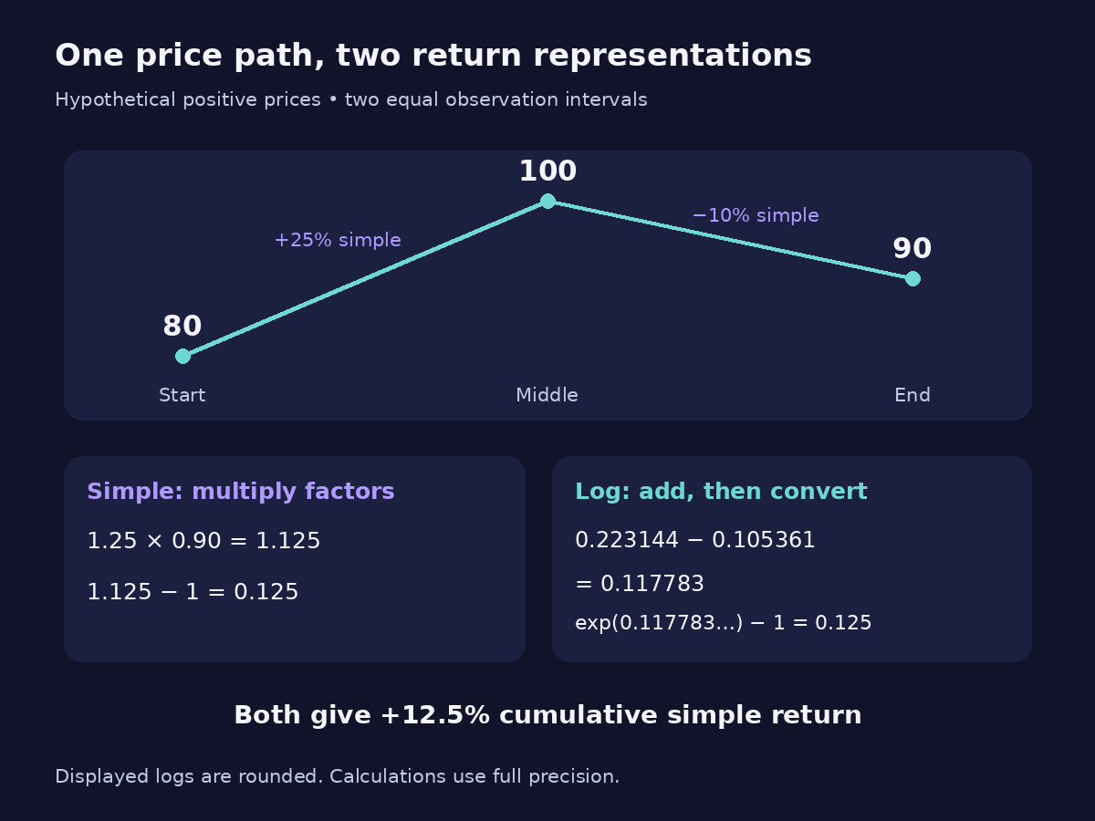
A fictional price rises from 80 to 100 and then falls to 90. Its two simple returns are +25% and −10%, but the overall gain is 12.5%. Add the corresponding logarithmic returns instead and you get a valid total in log units, which must then be converted back.
Simple vs log returns is a choice of mathematical representation. Both can describe the same positive-valued series. The useful question is how to calculate, combine and interpret each without accidentally switching units halfway through the work.
Simple vs log returns: define the two formulas
For positive prices P0 and P1, the simple return is R = P1 ÷ P0 − 1. The log return is r = ln(P1 ÷ P0), where ln means the natural logarithm. Returns are decimals in these formulas; multiplying by 100 expresses their reported numerical values in percent units.
The MathWorks price-to-return documentation distinguishes simple periodic returns from continuously compounded returns and makes the time-interval treatment explicit. For this article, each formula measures the complete stated observation interval. We do not divide it by elapsed days or call it an annual rate.
A simple return of 0.25 corresponds to a 25% gain in value. A log return of approximately 0.223144 corresponds to that same movement, often displayed as 22.3144% in log-return units. Calling the latter an ordinary 22.3144% gain would give the wrong ending value.
Use clear labels such as “simple return, %” and “log return × 100.” The percentage sign alone is insufficient to identify the transformation.
Calculate the same two-interval path both ways
Our hypothetical observations are 80, 100 and 90, recorded at equally spaced times. The series excludes distributions and other adjustments so the example focuses on transformation rather than income treatment.
In the first interval, the simple return is 100 ÷ 80 − 1 = 0.25, or +25%. In the second, it is 90 ÷ 100 − 1 = −0.10, or −10%.
The total simple return comes directly from the endpoints: 90 ÷ 80 − 1 = 0.125, or +12.5%. Adding 25% and −10% gives 15%, which does not reproduce the ending price. The second percentage acts on 100 rather than on the original 80.
The first log return is ln(100 ÷ 80) = approximately 0.223144. The second is ln(90 ÷ 100) = approximately −0.105361. Their sum is approximately 0.117783, equal to ln(90 ÷ 80).
Expressed as log return × 100, those values are +22.3144, −10.5361 and +11.7783. Keep more digits during computation than in the article display. Rounding each interval aggressively can create a small mismatch when the pieces are recombined.
Multiply simple growth factors; add log returns
To combine the simple returns, first turn each into a growth factor by adding one. The factors are 1.25 and 0.90. Multiply them: 1.25 × 0.90 = 1.125. Subtract one to recover the cumulative simple return of 12.5%.
Logarithms turn that multiplication into addition. The intermediate price cancels: (100 ÷ 80) × (90 ÷ 100) = 90 ÷ 80. Applying the logarithm gives the sum of the two interval log returns. The NIST identities for logarithms and exponentials provide the underlying mathematical relationship.
This additive property is across consecutive time intervals of the same consistently defined series. The intervals must join correctly. Adding overlapping weekly log returns, for example, can count the same days repeatedly.
Three prices produce two consecutive returns. A missing middle price does not stop you calculating the available endpoint return, but it does stop you observing the two separate movements. Adding a fictional flat observation to make the list look complete invents a path that the source did not record.
Convert before interpreting the result
The exact transformations are r = ln(1 + R) and R = exp(r) − 1. The exponential function reverses the natural logarithm. The NIST natural-logarithm reference describes that inverse relationship and the positive-number domain used here.
For the full example, exp(0.1177830357) − 1 = 0.125, or 12.5%. If instead you multiply 80 by 1 + 0.117783, you obtain about 89.42, which fails to recover the actual endpoint of 90. That is a unit error, not a different estimate of the same simple gain.
The two return measures are numerically close for small changes. A +1% simple return has a log return of about 0.9950% when multiplied by 100. A +50% simple return has a log return of about 40.5465%. The approximation becomes less comfortable as the move grows.
A −50% simple return has a log return of about −69.3147%. Do not use the +50% conversion with a minus sign: upward and downward simple percentages of the same magnitude represent different multiplicative factors.
Time additivity does not mean portfolio additivity
Consider a different hypothetical example. A portfolio starts with 50 currency units in asset A and 50 in asset B. Over one interval, A rises 20% and B falls 20%. Assume no external cash flows, costs or rebalancing during the interval.
A ends at 60 and B at 40. The portfolio still totals 100, so its simple return is zero. The beginning-value weighted simple returns agree: 0.5 × 20% + 0.5 × (−20%) = 0%.
Now take the same weighted average of the asset log returns. It is 0.5 × ln(1.20) + 0.5 × ln(0.80), approximately −0.020411. Converting that number gives about −2.0204%, which clearly does not describe the portfolio whose value remained 100.
The correct portfolio log return is ln(100 ÷ 100) = 0. To obtain it from component simple returns, first calculate the portfolio’s correctly weighted simple return, then apply ln(1 + R). The logarithm of a weighted sum is generally different from a weighted sum of logarithms.
This distinction matters when moving from one asset’s time series to a multi-asset dataset. A formula that aggregates correctly down the date column may not aggregate correctly across the asset columns.
Check the data and the domain before taking logs
The ordinary price-based log-return calculation in this guide requires positive prices at both ends. If a value is zero, the real logarithm is not finite. If a price crosses from positive to negative, the ratio is negative and this real-number log-return formula is unavailable.
A software function returning a result for two negative prices does not automatically give that result a sensible investment interpretation. The positive-value assumptions and the economic meaning of the input must both hold. Do not repair an unsuitable series by silently replacing values with small positive numbers.
Neither transformation cleans the data. A split, an inconsistent distribution adjustment or an incorrectly joined currency series can create a mechanical jump in simple and log returns alike. State the input definition before choosing the return formula.
For currency quotations, confirm the unit with the guide to base and quote currencies. For gaps, use missing market data versus zero. A missing observation is not a zero return, and a repeated stale price is not proof that a fresh market observation was unchanged.
Choose the representation that matches the question
Use a simple return when you want to describe a value change directly: “90 is 12.5% above 80.” Use log returns when the analysis benefits from adding consecutive transformed changes, while keeping the reported unit explicit. Neither representation creates evidence about the next movement.
For a statistical comparison, use the same representation throughout. Standard deviations, averages and fitted relationships can differ when the inputs are transformed. Do not take a statistic produced from log returns and relabel it as though its inputs were simple returns.
Time labels matter as much as the formula. A close-to-close return over three calendar days is a three-day interval even if the table places it beside several one-day observations. Decide whether your analysis concerns recorded observation intervals or standardised time units before pooling them.
Save the original price column, interval boundaries, transformation and final conversion in your market research journal. A small reproducible worksheet with those fields is enough to catch most accidental mixing of percentages, log units and growth factors.
Frequently asked questions
What is a log return in plain language?
It is the natural logarithm of the ending value divided by the starting value, for an appropriate positive-valued series. It represents the change in continuously compounded units and can be converted exactly to an ordinary simple return.
Are log returns more accurate than simple returns?
Both formulas can describe the same inputs exactly. They use different representations. Accuracy depends on correct data, arithmetic and interpretation, rather than one representation automatically being superior to the other.
Why can log returns be added across time?
Consecutive price ratios multiply and their intermediate prices cancel. The logarithm of that product equals the sum of the interval logarithms. This requires correctly joined, non-overlapping intervals in the same consistently defined series.
Can I add simple daily returns to get the monthly return?
Generally, no. Multiply each daily growth factor, one plus the simple return, then subtract one from the product. Addition can be an approximation for sufficiently small changes, but it is not the exact compounding calculation.
Does a 10% log return mean a 10% gain?
No. If the log return is 0.10, its simple equivalent is exp(0.10) − 1, approximately 10.5171%. A caption should state that the original figure is a log return before a reader interprets it as a change in value.
Can a log return be negative?
Yes. A positive price declining to a lower positive price produces a ratio between zero and one, whose natural logarithm is negative. Negative returns are valid here; zero or negative input prices raise a separate domain problem.
Why should I avoid averaging component log returns for a portfolio?
The assets combine through their values and beginning weights. A weighted average of their log returns generally differs from the logarithm of the portfolio growth factor. Our equal-weight +20% and −20% example demonstrates the mismatch.
Do log returns automatically include dividends?
No. Inclusion depends on the underlying data series. Logging an unadjusted price ratio does not add an omitted distribution. Decide whether the research requires a price-return or total-return series before applying the transformation.
Which logarithm should I use?
For the conventional log returns described here, use the natural logarithm, often written ln. A base-10 logarithm gives different numerical units. Check the software documentation because function names such as log can vary across tools.
What should I do after summing log returns?
If the audience needs an ordinary cumulative percentage gain or loss, apply exp to the sum, subtract one and multiply by 100. Preserve the interval dates and input basis so the converted result remains a clearly defined measurement.
Educational information only. All worked numbers are hypothetical unless identified as a source definition. This article provides no forecast, recommendation or investment advice.