

Portfolio diversification depends on the exposures held, their sizes and how their returns move together. Counting the number of tickers or funds is only a starting point. Two portfolios with identical holdings can have different variability because their weights differ.
This guide connects portfolio weights, volatility and covariance through a transparent two-asset example. It also examines overlapping fund holdings and the limits of a historical correlation estimate. The examples are hypothetical teaching devices, not suggested allocations.
Portfolio diversification needs more than a holding count
Diversification spreads exposure across investments. Its volatility effect comes from combining return streams that do not move in perfect step, subject to their weights and individual variability. The two-asset calculation below makes the role of each input explicit.
A portfolio containing ten tiny positions and one dominant position can remain concentrated. Several funds can also hold the same underlying companies or respond to the same sector, currency or interest-rate exposure.
Consequently, an informative description names the portfolio boundary and measurement basis. “Twelve holdings” is an inventory fact. “A large share of the portfolio depends on the same issuer or economic exposure” is a separate concentration question.
Separate weights, volatility, correlation and covariance
A weight is an asset’s share of portfolio value. In the simple unlevered examples here, the two weights are positive and add to one. A 60% weight is entered into calculations as 0.60.
Volatility here means the standard deviation of a return series over a stated horizon. A 20% annual standard deviation is represented as 0.20. It is a measure of variability, not a maximum possible loss.
Correlation standardizes co-movement between return series on a scale from −1 to +1 when it is defined. Covariance retains the scale of the returns. For assets A and B:
Covariance(A,B) = correlation(A,B) × volatility(A) × volatility(B).
Correlation alone does not supply the covariance. A correlation of 0.25 between two highly variable assets gives a different covariance from 0.25 between two relatively stable assets. Both the standard deviations are needed.
CFA Institute’s worked diversification explanation sets out the corresponding variance calculation. The focus here is its application to portfolio composition, rather than using correlation to establish a causal relationship.
Hypothetical example: build the covariance term
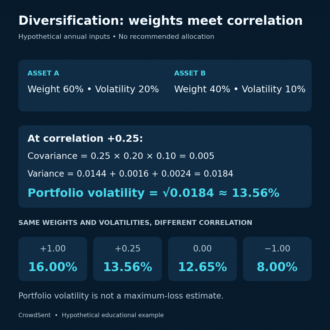
Assume a two-asset portfolio with these invented inputs, all measured on the same annual basis:
- Asset A: 60% portfolio weight and 20% volatility.
- Asset B: 40% portfolio weight and 10% volatility.
- Correlation between A and B: +0.25.
The covariance is 0.25 × 0.20 × 0.10 = 0.005. For fixed weights, portfolio variance equals:
wA2σA2 + wB2σB2 + 2wAwBCov(A,B).
Insert the assumptions one term at a time:
- A’s weighted variance term: 0.602 × 0.202 = 0.0144.
- B’s weighted variance term: 0.402 × 0.102 = 0.0016.
- The cross term: 2 × 0.60 × 0.40 × 0.005 = 0.0024.
Total variance is 0.0184. Taking the square root gives portfolio volatility of approximately 0.13565, or 13.56%.
The simple weighted average of the asset volatilities would be 0.60 × 20% + 0.40 × 10% = 16%. That shortcut omits the actual co-movement structure. It equals the portfolio volatility in this positive-weight example only when correlation is +1.
Notice another important comparison: 13.56% is below 16%, but above B’s standalone 10% volatility. Diversification does not mean the combination must be less variable than every asset it contains.
Change correlation while holding everything else fixed
A controlled sensitivity calculation changes just one input. Keep the 60/40 weights and the 20% and 10% volatilities, then substitute different correlations:
- At correlation +1.00, portfolio volatility is 16.00%.
- At correlation +0.25, it is approximately 13.56%.
- At correlation 0.00, it is approximately 12.65%.
- At correlation −1.00, it is 8.00%.
Zero correlation makes the cross term zero, but leaves the two weighted variance terms. It therefore does not make the portfolio risk-free.
Even perfect negative correlation does not produce zero variability with these weights. At −1, portfolio volatility simplifies to the absolute difference between weighted volatilities: |0.60 × 20% − 0.40 × 10%| = 8%.
For this special theoretical case to cancel completely, the weighted volatilities would need to match. That algebraic condition is not evidence that real assets maintain perfect negative correlation or stable future volatilities.
Change the weights while keeping correlation unchanged
Now return to correlation +0.25 and change the hypothetical portfolio to 90% A and 10% B. The variance becomes:
0.902 × 0.202 + 0.102 × 0.102 + 2 × 0.90 × 0.10 × 0.005 = 0.0334.
Its square root is approximately 18.28%. The portfolio still has two assets and the same pairwise correlation, yet its measured variability is higher than in the 60/40 example because more weight sits in A.
This portfolio diversification comparison is intentionally narrow. It does not establish an appropriate allocation: expected returns, liabilities, costs and personal constraints are outside the example. It establishes only that holding count and correlation do not determine portfolio volatility without the weights.
Look through funds to measure overlapping exposure
Consider a separate hypothetical portfolio with 75% in Fund F and 25% directly in Company X. Assume Fund F itself has 20% of its assets in Company X.
The fund creates an indirect X exposure of 75% × 20% = 15% of the overall portfolio. Add the direct 25% holding and total X exposure is 40%.
A statement showing two line items could therefore hide a substantial common issuer exposure. Adding another fund with a similar X holding could add a third line item without reducing that overlap.
FINRA’s concentration-risk guidance discusses correlated holdings, fund overlap and concentration that develops as asset values change. For an exposure review, the relevant evidence is the underlying holdings and their dates, not just the product names.
Weights can drift even without a transaction. In a hypothetical 50/50 portfolio, if A doubles while B is unchanged, their values move from 50 and 50 to 100 and 50. A’s new weight is two-thirds. A risk calculation that still uses the original 50/50 weights no longer describes that ending portfolio.
Portfolio diversification: limits of historical correlations
Correlation is estimated from a chosen sample and frequency. Daily and monthly return observations need not produce identical estimates. Currency conversion, unsynchronized market closes and missing prices can also change the input series.
The Bank for International Settlements’ research on equity and bond correlations illustrates that relationships can change across economic conditions. An asset-class label is therefore not a permanent correlation setting.
A stress calculation can show what the same portfolio would look like under alternative assumed correlations or volatilities. It is a sensitivity exercise, not a probability forecast. Changing correlation while fixing everything else is useful for understanding the formula; real episodes can change several inputs together.
Standard deviation also leaves out important dimensions. It does not tell us whether assets can be sold at the displayed price, whether financing is available or whether an unusual joint loss will occur. CrowdSent’s liquidity-versus-volume guide provides a separate lens on execution conditions.
As the SEC’s diversification explanation makes clear, spreading investments cannot guarantee protection from losses when markets decline.
A portfolio diversification measurement checklist
- Define the portfolio boundary, valuation date and reporting currency.
- Reconcile weights to the included assets and cash.
- Look through funds and derivatives for overlapping exposures.
- Match the return window, frequency and currency across assets.
- Calculate covariance using consistent volatility and correlation inputs.
- Separate the base calculation from alternative-input scenarios.
- Record liquidity, concentration and data limitations alongside volatility.
For input checks, see missing market data versus zero. Keep assumptions and results together in a research journal.
Frequently asked questions
1. Does owning more funds always improve diversification?
No. Additional funds can repeat existing holdings or economic exposures. Their underlying assets and weights determine whether the portfolio’s exposure pattern meaningfully changes.
2. Is negative correlation required for a diversification effect?
No. In the positive-weight example, correlation of +0.25 already produces volatility below the weighted average of the standalone volatilities. Perfect negative correlation is a special theoretical case.
3. Why are weights squared in the variance terms?
Scaling a return by a weight scales its variance by the square of that weight. The cross term then accounts for the covariance between the two weighted return contributions.
4. Why is the covariance term multiplied by two?
Expanding the square of a sum produces two matching cross-products. For two assets, those products combine into 2 × weight A × weight B × covariance.
5. Does zero correlation mean the assets cannot fall together?
No. Zero correlation is a statement about measured linear co-movement over a distribution or sample. It does not prohibit a particular joint negative outcome.
6. Can diversification reduce risk below both assets’ volatilities?
It can for some inputs, but it is not guaranteed. In the main example, portfolio volatility of 13.56% remains higher than B’s 10% standalone volatility.
7. Are equal capital weights equal risk contributions?
Not generally. Different volatilities and covariances mean equal dollar allocations can affect portfolio variability differently. A 50/50 value split does not establish a 50/50 risk split.
8. Can I reuse old weights with current covariance estimates?
Only if the intended analysis uses those old weights as a stated scenario. To describe a current portfolio, use its relevant current exposures and disclose the estimation window.
9. Does the simple formula cover leveraged portfolios?
The covariance framework can accommodate signed and leveraged exposures, but weights, financing and instrument behavior need careful definition. The unlevered examples here do not model those additional complications.
10. Does lower calculated volatility guarantee a smaller future loss?
No. The calculation depends on inputs and measures variability rather than a loss limit. Concentration, liquidity and changing relationships remain relevant even when the estimated standard deviation is lower.
To explore the workspace and its membership options, open CrowdSent.
Educational note: These calculations illustrate portfolio measurement. They are not allocation recommendations, individualized investment advice or guarantees against loss.