

By CrowdSent Blog Team
Impermanent loss is the shortfall between a liquidity position’s value and the value of simply holding its original assets, measured at the same later prices. The classic calculation isolates the effect of the pool’s changing asset mix. Fees, incentives and transaction costs need separate treatment.
This comparison is easy to misunderstand because a position can rise in dollar value and still have impermanent loss. The benchmark also rises, and may rise by more. The word “loss” therefore needs both a denominator and a clearly defined alternative.
This guide works through a hypothetical two-asset, full-range, 50/50 constant-product pool. It explains the arithmetic, the meaning of “impermanent” and the limits of applying this model to other pool designs. No example is a live price, return forecast or recommendation.
Impermanent loss starts with the holding benchmark
The benchmark is the original quantities of both assets held unchanged. It is not the value of holding only the asset that subsequently performs best, and it is not automatically the original dollar deposit.
Suppose the starting assets are 1 A and 100 B. At a hypothetical price of 100 B for one A, the two components have equal value. If B is valued at $1 for the example, the starting portfolio is worth $200.
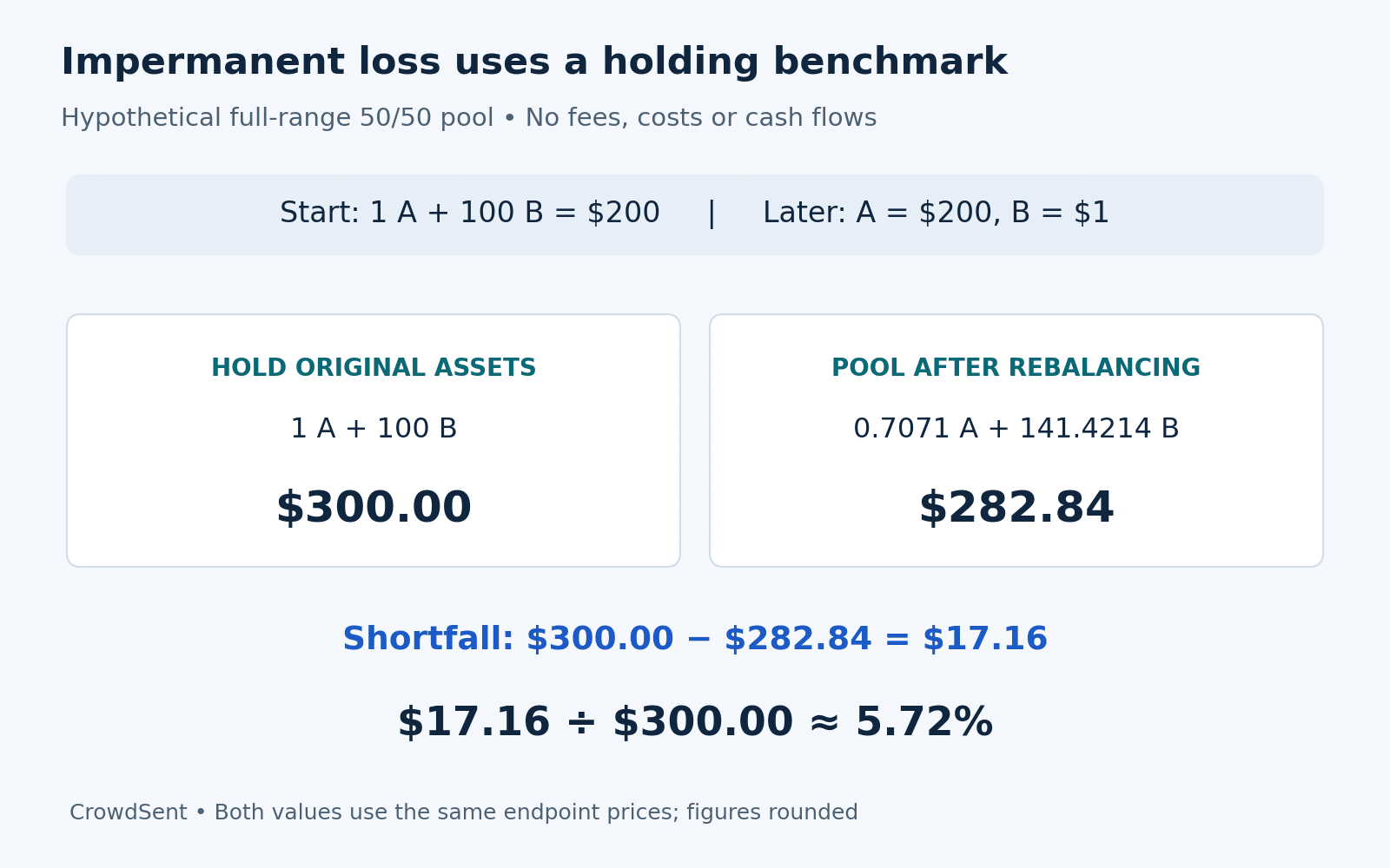
At a later A price of 200 B, the unchanged portfolio would contain the same 1 A and 100 B, worth $300. That $300 is the comparison value for this endpoint. A liquidity position should be valued at exactly the same endpoint prices.
Uniswap’s v2 discussion of liquidity-provider returns explains the comparison with holding and how reserve adjustment produces it. The article’s own example below uses different numbers and explicitly excludes fees to expose the mechanism.
Why the pool ends with different asset quantities
For the simplified constant-product position, the starting quantity product is 1 A multiplied by 100 B, or 100. When the external relative price changes, arbitrage is assumed to align the pool with that price without fees or other frictions.
At the endpoint, two conditions hold in the model: A quantity multiplied by B quantity remains 100, and B quantity divided by A quantity is 200. Solving them gives approximately 0.7071 A and 141.4214 B.
The pool now contains less of the asset that became relatively more expensive and more of the other asset. This changing composition is the source of the benchmark shortfall. The calculation does not require a hack, a failed transaction or an explicit withdrawal charge.
A complete worked calculation
Value the pool position at the endpoint: 0.7071 A multiplied by $200 is about $141.42. Add $141.42 for the B component. The position is worth approximately $282.84 before fees and costs.
Holding the original 1 A and 100 B would be worth $300. Subtracting $282.84 from $300 gives a shortfall of about $17.16. Dividing that gap by the $300 holding benchmark gives approximately 5.72%.
The liquidity position rose from $200 to $282.84, a gain of about 41.42%. The unchanged holding rose from $200 to $300, a gain of 50%. Both statements can be true alongside 5.72% impermanent loss.
Notice that 50% minus 41.42% is 8.58 percentage points, not 5.72%. The percentage-point return gap uses the original $200 denominator. The standard impermanent-loss percentage uses the final $300 benchmark. Explicit denominators resolve the apparent contradiction.
The familiar formula and its assumptions
Let r be the final price ratio divided by the initial price ratio for A measured in B. In the fee-free, full-range, 50/50 constant-product model, the liquidity position’s value divided by the holding benchmark is 2 times the square root of r, divided by 1 plus r.
Subtract 1 to express the result as a signed relative difference. When r equals 2, the result is about minus 5.72%. A calculator that displays “5.72% loss” is expressing the positive magnitude of the same shortfall.
This compact formula depends on the model. It assumes the original deposit is balanced by value, the position remains full range, no liquidity is added or removed during the comparison, and reserves adjust to the endpoint price. Fees and costs are excluded.
It also depends on the assets’ relative price. If both rise in the same proportion against the dollar, their exchange ratio is unchanged. In this idealized model, that common dollar move alone does not create the composition effect measured by the formula.
What happens when the relative price falls?
Use the same starting 1 A and 100 B, but let A fall from $100 to $50 while B stays at $1. The pool quantities become about 1.4142 A and 70.7107 B. Their combined value is approximately $141.42.
The unchanged holding would be worth $150: $50 of A plus $100 of B. The shortfall is about $8.58, again 5.72% of the endpoint holding value.
The percentage symmetry comes from a doubling and a halving being reciprocal price-ratio moves. The dollar shortfalls differ because the benchmark values differ. This is why an impermanent-loss percentage should not be read as a fixed dollar charge.
Here, both the pool position and the holding benchmark lost value from the original $200. Separating absolute performance from relative performance is essential. CrowdSent’s guide to crypto price and valuation measures offers related context on avoiding conclusions from a single number.
What “impermanent” does and does not mean
In the unchanged, fee-free model, the composition shortfall returns to zero if the pair’s relative price returns to its starting ratio. That possibility explains the term. It does not establish a deadline or a guarantee that the price will return.
The comparison exists while the position remains open. Redeeming the position records the asset mix available at that point, but a visible shortfall does not wait for redemption before it matters economically.
Once cash flows, fees, position changes or different ranges enter the history, returning to an earlier price is not enough to reconstruct performance with the simple endpoint formula. The relevant analysis must include what actually happened to the position.
“Divergence loss” is another term readers may encounter for this composition effect. Whichever label a source uses, check its definition and benchmark before comparing its number with a different calculator.
How fees and incentives affect the comparison
Fees can offset a benchmark shortfall, but their presence does not prove that they did. In the doubling example, the fee-free gap is $17.16. A hypothetical net additional value greater than that gap would change the comparison, provided it is genuinely incremental and measured consistently.
Actual fee accounting is more involved than adding a headline annual percentage. Fees can accumulate in the underlying assets, change the position’s composition or be held separately. Incentive tokens have their own quantities and endpoint prices. Costs must be placed on the same basis.
Most importantly, do not add fees twice. If fees already increase the pool reserves used to value the position, adding the same fee total again overstates performance. A clean comparison reconciles the full position value, separate distributions and cash flows.
Network costs are a distinct line item. CrowdSent’s explanation of Ethereum gas fees helps distinguish them from pool fees. None of these calculations requires assuming that a quoted incentive or recent activity level will continue.
Where the standard formula stops working
A concentrated-liquidity position has specified range boundaries. Its asset composition and active status depend on those boundaries as well as the current price. An out-of-range position may consist entirely of one asset, so the full-range formula is insufficient.
The official Uniswap concentrated-liquidity documentation describes this range-dependent behavior. Applying a generic 50/50 calculator without position bounds can produce a number for a different exposure than the one being studied.
Weighted pools also require their own treatment. Balancer’s weighted-pool mathematics documentation makes the dependence on asset weights explicit. Stable-asset designs and pools with custom behavior similarly need their actual invariant and accounting.
These model differences are separate from technical safety. A correct impermanent-loss calculation does not assess every way a position could lose value. Ethereum’s smart-contract security documentation covers a different category of risk.
Record the comparison before interpreting the percentage
A reproducible note identifies the original token quantities, start and end timestamps, price sources, pool design, cash flows and fee treatment. It states whether the result is the simplified composition effect or actual performance relative to holding.
If an input is unavailable, leave the result qualified rather than filling the gap with zero. CrowdSent’s missing-data guide explains the broader reporting problem. An exact-looking percentage cannot repair uncertain inputs.
Frequently asked questions about impermanent loss
1. Can impermanent loss occur while a position gains value?
Yes. It measures performance against holding the original assets at the same endpoint prices. A position can rise in value while the unchanged holding rises more. The worked example produces a positive dollar return alongside a 5.72% benchmark shortfall.
2. Is the comparison against holding only one token?
The classic benchmark holds the original quantities of both deposited assets. Replacing that benchmark with only the better-performing token answers a different question. A calculator should state its benchmark clearly so its result can be interpreted and reproduced.
3. Why does a 100% price increase produce about 5.72% loss?
The 100% change describes one asset’s price relative to the other. The 5.72% compares the rebalanced pool position with an unchanged two-asset portfolio. These are different measurements with different denominators, linked by the constant-product model rather than by subtraction.
4. Is impermanent loss charged as a separate fee?
No. In the classic example, it emerges from the different asset quantities held by the pool after the relative price changes. There is no separate 5.72% deduction. Transaction and protocol charges, where applicable, belong in additional accounting lines.
5. Does waiting guarantee that the shortfall disappears?
No. The fee-free model’s shortfall disappears if the relative price returns to its starting ratio, but there is no guarantee of that return. Changes to the position and its cash flows also complicate the comparison beyond the simple model.
6. Can stablecoin pools experience this effect?
A stable label does not fix the exchange ratio forever. Assets can diverge from their intended relationship, and different pool curves respond differently. A stable-asset pool should be evaluated using its actual design and observed prices rather than assuming the composition effect is always zero.
7. Does high trading volume prove fees cover the shortfall?
No. Fee rates, the position’s share of active liquidity, protocol deductions, price changes and costs all matter. Volume alone cannot establish net performance. Even a pool-wide fee total may not identify what a particular position earned over the same interval.
8. Can I use the same formula for an 80/20 pool?
No. The familiar square-root formula assumes equal starting value weights. A different weighting changes the mathematical relationship between the pool and holding benchmark. Use the weighted design’s formula and preserve its assumptions when interpreting the result.
9. Does withdrawal create impermanent loss?
The relative shortfall can already exist in an open position. Withdrawal determines the quantities received at that time under the contract’s rules. It does not retroactively create the composition changes that produced the comparison with holding.
10. What should a reliable calculator disclose?
It should identify the pool model, starting quantities or weights, endpoint prices, range boundaries where relevant, and treatment of fees and costs. It should also show the holding benchmark and denominator. Without those details, identical labels can hide incompatible calculations.
Conclusion: keep the benchmark in view
Impermanent loss becomes clearer when the original holding and the changing pool position are valued side by side. The central questions are which asset mix changed, which benchmark was used and what the percentage divides by. Fees, ranges and cash flows then determine how far the simple model can be extended.
This guide is an educational reference for evaluating liquidity-position explanations and their assumptions.
Source documentation checked 11 October 2026. Educational explanation from the CrowdSent Blog Team. Numerical examples are hypothetical unless explicitly identified otherwise. This article does not provide investment recommendations.