

Correlation and causation answer different questions. Correlation describes how two measured series vary together in a particular dataset. A causal claim says that changing one factor would change another through a specified mechanism. Finding a relationship on a market chart is a starting point for investigation, not proof of that mechanism.
This distinction becomes especially useful when a price rise, a burst of online discussion and a news announcement happen close together. Any two may be associated, while a third event helps explain both. A careful research note preserves what was measured, how the comparison was built and which explanations remain unresolved.
Correlation and causation answer different questions
Pearson’s correlation coefficient summarises a linear relationship between paired observations. It ranges from −1 to +1 when defined. Positive values describe a tendency for the two measurements to be above or below their respective sample averages together. Negative values describe a tendency for them to move in opposite directions relative to those averages.
The NIST correlation reference sets out the coefficient and its linear interpretation. A value near zero means little measured linear association in that sample; it does not rule out every nonlinear relationship. If one series is constant, the usual coefficient is undefined because there is no variation in that series to standardise.
For a fictional five-period example, let asset A’s returns be +1%, −1%, +2%, −2% and 0%. Let asset B’s returns be +2%, −2%, +4%, −4% and 0%. Every B observation is twice its paired A observation, giving a Pearson correlation of +1.
That calculation says nothing about who or what caused the returns. Both assets could be responding to a shared announcement. The numbers might even have been constructed by an analyst, as they were here. The coefficient cannot distinguish those explanations from the pairs alone.
A shared cause can produce a persuasive market story
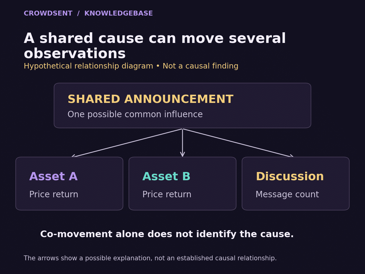
Imagine a fictional announcement that changes expectations about demand in an industry. Asset A and asset B are both exposed to that industry. Discussion volume about both also rises because people are responding to the same announcement. A chart may show all three moving together.
One possible explanation is that the announcement influenced prices and discussion separately. Another is that prices moved first and attracted attention. A further possibility is that some participants anticipated the announcement, so both prices and posts began changing beforehand. None is established simply by overlaying the lines.
The NIST scatter-plot guide explains that a visible association does not by itself establish cause and effect. In a research note, use that distinction literally: write “the measures were associated in this sample” until the design supports a more specific claim.
To move beyond that description, ask what evidence would distinguish the explanations. You might need original publication times, the information available beforehand, comparable observations without the event and a clear mechanism. Even then, the conclusion must match the strength and limitations of the research design.
Decide whether you mean prices, changes or returns
The phrase “these markets are correlated” leaves the measured variable unspecified. Are you comparing price levels, changes in currency units, percentage returns, trading volume or sentiment scores? Those choices can produce different answers and address different questions.
For a simple return, divide the new price by the previous price and subtract one. If a fictional price moves from 100 to 102, the return is 2%. If another moves from 50 to 51, its return is also 2%, although the currency-unit changes are different. This normalisation makes the comparison about proportional changes.
Long price-level series can share a broad upward or downward direction even when their short-period changes have a different relationship. A price-level correlation therefore needs a reason grounded in the research question. It should not be casually described as evidence that day-to-day returns move together.
Consider two fictional three-observation paths: A moves from 100 to 110 to 105, while B moves from 50 to 48 to 55. Both finish above where they started. Yet their first returns have opposite signs, and their second returns also have opposite signs. A shared start-to-finish direction misses the paired interval behaviour.
For a return comparison, document the currency, adjustment convention and treatment of distributions. A price-only stock series and a total-return series answer different measurement questions. If a currency conversion is applied to one series, the resulting returns include that conversion’s effect. Keep the choice consistent or explain the intended difference.
Pair the same periods before calculating anything
Each point in the correlation calculation is a pair. If A’s observation refers to one period and B’s refers to another, the result measures the relationship between those mismatched pairs. A correct formula cannot repair an incorrectly assembled sample.
Suppose A’s daily return ends at a fictional 16:00 UTC, while B’s daily return ends at 21:00 UTC. An announcement at 18:00 can affect B’s recorded day while falling outside A’s corresponding window. Pairing the observations by calendar date may obscure this difference.
The same problem appears when one market is closed and another continues updating. Carrying a previous value forward creates a recorded zero change, but that may represent an unobserved fresh price rather than a genuine new observation. The guide to missing market data versus zero helps distinguish those cases.
Keep a written rule for holidays, missing values and unequal update frequencies. List how many complete pairs survive. If you compare daily prices with a weekly discussion measure, first define which daily observations contribute to each weekly window. Otherwise the result may depend more on your joining rule than on the relationship you wanted to study.
Why the sample and rolling window change the answer
A coefficient belongs to a dataset and a period. Five hypothetical pairs can demonstrate arithmetic, but they provide little basis for describing a persistent market relationship. Adding more observations can change the result, especially if the original sample concentrated on one unusual episode.
A rolling correlation repeats the calculation over a moving window. A 20-observation version keeps the most recent 20 valid pairs under its defined rule, then shifts as another pair arrives. A 60-observation version includes a longer history. Neither number is automatically the correct choice for every question.
Imagine 19 moderate observations and one unusually large joint move. When that extreme pair enters a 20-observation window, it can materially affect the coefficient. When it later drops out, the rolling value may change sharply even if the newest pair is ordinary. Look at the entering and departing observations before inventing a new market narrative.
Adjacent rolling windows share most of their data. Twenty consecutive chart points from a 20-observation rolling calculation are not twenty independent studies of the relationship. Keep that overlap in mind when describing how much evidence a smooth-looking chart contains.
Sample selection matters too. If you try dozens of start dates and report only the strongest coefficient, the final number hides the search that produced it. Define a main comparison in advance, show relevant alternative windows and preserve an honest record of tests that did not support the initial idea.
Inspect the relationship rather than just the headline number
Plot the paired observations and label the axes with the actual variables and units. Look for an isolated extreme pair, groups from different periods and a curved relationship that one linear coefficient would summarise poorly. Keep the original records available so unusual points can be checked against their sources.
Do not remove an inconvenient point just because it changes the conclusion. First establish whether it is an error, a measurement change or a real observation. If you present a sensitivity calculation without it, show the full-sample result as well and explain the exclusion rule.
Keep uncertainty separate from causality. A statistical test can assess a claim about association under stated assumptions; a small probability under a null model does not supply a causal mechanism. Financial time series also need an inference method suited to their time dependence rather than an automatic assumption that every observation is independent.
If the comparison involves a sentiment measure, inspect how that measure is constructed before interpreting it. A change in coverage or scoring can change the series without an equivalent change in underlying opinion. What a sentiment score means explains why polarity, confidence and evidence should be kept distinct.
Write a conclusion another researcher can check
A useful conclusion names the variables, sources, observation windows, number of paired records, transformation and sample dates. It gives the measured coefficient if you calculated one and identifies unresolved alternatives such as a common driver, reverse direction or timing mismatch.
For the fictional five-pair example, a suitable statement is: “A and B’s constructed returns have a correlation of +1 across these five pairs. B is exactly twice A by design. The example demonstrates linear association and contains no evidence about a real market or causal effect.”
For actual research, save the setup before looking at further data and distinguish exploratory findings from a separately evaluated result. The market research journal template can help retain the original question, contrary evidence and revisions without rewriting the story after seeing the outcome.
Frequently asked questions
What is the difference between correlation and causation?
Correlation describes an association between measurements. Causation concerns whether a change in one factor produces a change in another through a supported mechanism. The first can be measured from paired data without establishing the second.
Does a correlation of +1 prove a cause?
No. It describes a perfect positive linear relationship in the sample when the coefficient is defined. A shared driver, a construction rule or another explanation can produce that relationship without either variable causing the other.
Does zero correlation mean two variables are unrelated?
Zero Pearson correlation means no measured linear association in the sample. A nonlinear relationship may still exist. Inspect the data and the question being asked rather than treating one coefficient as a complete description.
Should I compare returns instead of prices?
For questions about proportional market changes, aligned returns are often the relevant measurement. A price-level question may require levels. State the choice explicitly because the two calculations describe different relationships.
Can positive correlation include opposite moves on some days?
Yes. A positive sample coefficient does not require every paired return to have the same sign. It summarises how the full set of observations varies around the respective sample averages.
What is a confounder in a market comparison?
It is a factor that can help explain both measurements and complicate an asserted causal relationship between them. A shared announcement affecting two assets is a simple hypothetical example. Identifying one requires evidence beyond coincidence.
Does moving first prove that a series causes another?
No. The apparent lead could reflect different observation windows, publication delays or anticipation of a common event. A consistent time order may be relevant to a causal investigation, but it is not sufficient on its own.
Why does rolling correlation change?
New pairs enter the window and older pairs leave. The relationship, composition, data quality or influence of an extreme observation may change. Check the underlying pairs before attributing every movement to a new economic regime.
Is a statistically significant correlation causal?
No. Significance concerns a statistical comparison under assumptions. It does not by itself resolve shared causes, reverse direction, selection effects or measurement timing. Causal language requires evidence from the research design.
Can a historical correlation predict the next price move?
The historical coefficient describes the selected observations. A predictive claim needs its own defined evaluation and may fail when conditions or data construction change. Do not convert a descriptive relationship into a guaranteed next-period direction.
A careful market comparison begins with a precise variable and a well-aligned sample. Correlation can summarise that evidence. Keep explanations, causal claims and future expectations separate until each has been supported by the appropriate additional work.