Seasonally Adjusted Data: Factors, Comparisons and Revisions

What seasonally adjusted data is designed to show

Seasonally adjusted data removes an estimate of recurring seasonal influences from a time series. The aim is to make nearby periods easier to compare when predictable calendar patterns would otherwise dominate the movement.

The BLS seasonal-adjustment FAQ gives examples such as weather patterns, production cycles, holidays, and sales. The adjustment is statistical: it does not mean the original activity or prices never happened.

Imagine a shop whose sales usually increase during a particular holiday period. Observing a rise then answers “Did sales increase?” A seasonally adjusted comparison asks a further question: how did the movement compare with the estimated recurring pattern for that time of year?

Those questions can produce different signs without a contradiction. Activity can increase but less than the seasonal pattern would suggest. A simple invented example below shows the arithmetic.

This guide uses US statistical documentation as its reference. The classroom shop is fictional and has no country-specific seasonal pattern. Readers in India and Pakistan should use the relevant domestic publisher’s methods rather than assuming a US holiday calendar applies to their data.

Worked example: a seasonal rise with no adjusted growth

Suppose a fictional sales series has November sales of 1,100 units and December sales of 1,250. Assume known multiplicative seasonal factors of 1.10 for November and 1.25 for December. We supply these factors to demonstrate the calculation; two observations cannot estimate a reliable seasonal model.

In a multiplicative setup, the adjusted value is the original value divided by its factor. The US Census Bureau’s seasonal-adjustment explanation describes this approach and distinguishes it from additive adjustment, which subtracts an estimated seasonal amount.

• November adjusted: 1,100 ÷ 1.10 = 1,000.
• December adjusted: 1,250 ÷ 1.25 = 1,000.
• Unadjusted growth: 1,250 ÷ 1,100 − 1 ≈ 13.64%.
• Adjusted growth: 1,000 ÷ 1,000 − 1 = 0%.

The shop sold 150 more units in December. The adjusted series nevertheless shows no growth because the seasonal factor is proportionately higher. Both descriptions are correct under the example’s assumptions.

A factor of 1.25 means the unadjusted level is 1.25 times the adjusted level in this simplified decomposition. It does not mean subtract 25% from the original value. Doing that would produce 937.5, while division correctly gives 1,000.

That distinction is easy to miss when a spreadsheet displays a factor as 125. If the source expresses the factor on a 100-based scale, first interpret that convention correctly. Our formulas use factors of 1.10 and 1.25, not 110 and 125.

Why adjusted and unadjusted data can move in opposite directions

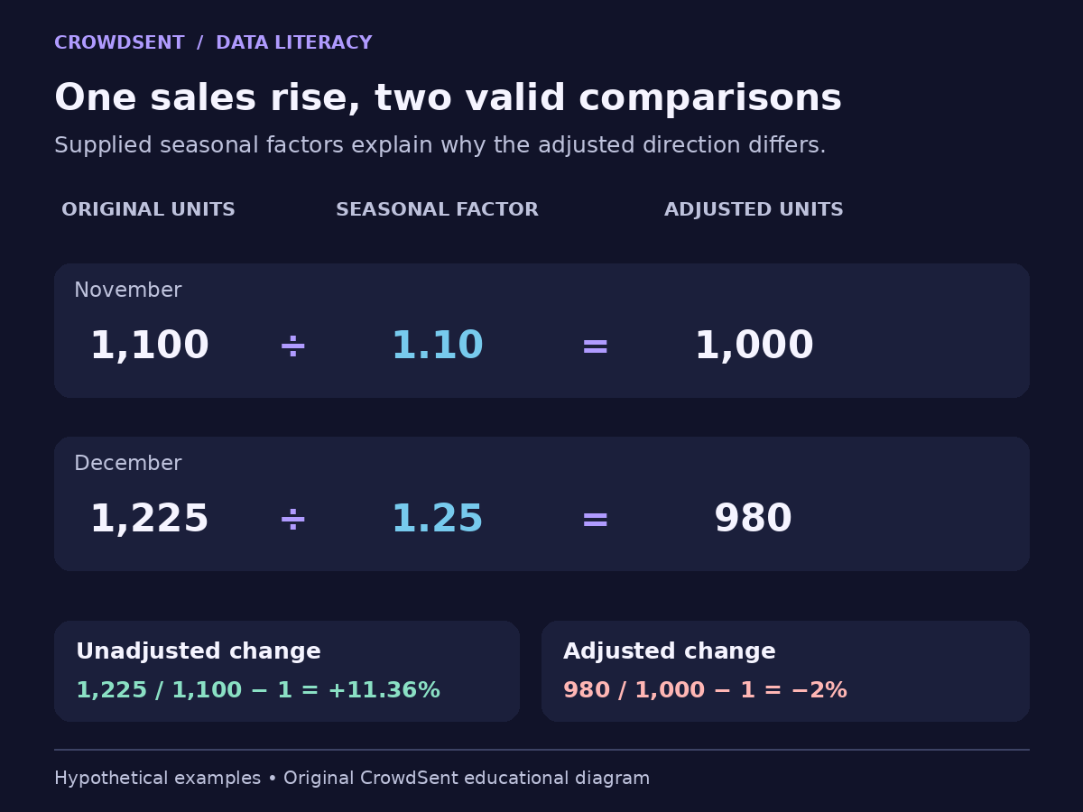
Now change December sales to 1,225 while leaving November at 1,100 and both seasonal factors unchanged. Unadjusted sales still rise: 1,225 ÷ 1,100 − 1 ≈ 11.36%.

December’s adjusted level is 1,225 ÷ 1.25 = 980. Compared with November’s adjusted 1,000, this is a decline of 2%. The seasonal increase in observed sales is smaller than in the previous scenario.

A careful description is: “Hypothetical sales rose 11.36% before seasonal adjustment and fell 2% after applying the stated factors.” Avoid saying sales “really fell” without explaining the adjustment. The two numbers answer different questions about the same supplied observations.

It would also be wrong to call the 2% decline the number of units lost. A percent change is relative to the adjusted base. The actual unit count increased by 125, while the adjusted level decreased by 20 in the model.

For an audit, reverse the calculation. Multiplying December’s adjusted 980 by its factor of 1.25 returns 1,225. Multiplying November’s adjusted 1,000 by 1.10 returns 1,100. Both endpoints can be reconstructed.

This reverse check is especially useful when a downloaded file includes original values, factors, and adjusted results in neighbouring columns. It can reveal a scale error before the analyst writes an explanation.

Choose the version that fits the question

Seasonal adjustment is useful when the question concerns a recent movement after accounting for recurring timing patterns. The original series remains useful when the question concerns the observed level or an application explicitly defined using unadjusted data.

For US CPI, BLS guidance on adjusted and unadjusted data says adjusted changes are generally preferred for analysing short-term price trends. It also explains that unadjusted indexes are commonly used for escalation arrangements, because seasonally adjusted series are revised.

That is a reason to read the named series in an agreement or source document, not a recommendation to substitute one series into an existing contract. The label is part of the specification.

A shop manager asking how many units need storage in December needs the relevant operational quantity. A researcher asking whether sales strengthened beyond the recurring December pattern needs a different comparison. Neither purpose makes the other dataset false.

Annual comparisons also need their own label. Comparing December with the previous December can reduce some recurring month effects, but it is not identical to a formal seasonal adjustment. Nor is it the same as comparing the latest two adjusted months.

Adjustment does not remove every source of variation

An adjusted series can still contain irregular movements. Removing a recurring seasonal estimate is not the same operation as smoothing every fluctuation, removing inflation, or forecasting the next observation.

Suppose the fictional shop loses two trading days because of an unexpected local event. Our supplied factors contain only the assumed recurring pattern. Dividing by 1.25 would not identify that event or tell us what sales would have been without it.

Statistical methods may treat unusual observations specially when estimating seasonal patterns. BLS’s explanation of intervention analysis describes handling outliers and level shifts before estimating some CPI seasonal factors, so unusual events do not distort the recurring pattern.

The purpose is not to claim that an unusual price movement never occurred. Distinguish estimating the seasonal component from deciding how the resulting adjusted observations should be interpreted.

Also keep seasonal adjustment separate from inflation adjustment. A seasonally adjusted sales value expressed in current money can still change because prices changed. “Adjusted” is incomplete unless the writer says what was adjusted for.

For a chart caption, use full terms such as seasonally adjusted sales units or seasonally adjusted current-currency sales. An unexplained “real” or “clean” series makes the transformation harder to audit.

A revised factor can change an old adjusted value

Seasonal patterns are estimated, and later information can change those estimates. For US CPI, BLS normally recalculates factors annually and can revise seasonally adjusted indexes for the preceding five years. Other statistical programs have their own policies.

Return to the 1,225-unit December scenario. With a factor of 1.25, the adjusted level is 980. Suppose a later methodology update in this toy example revises that factor to 1.225. Holding the observed 1,225 unchanged, the revised adjusted level is 1,000.

If November stays at an adjusted 1,000, the previously calculated −2% movement becomes 0%. No additional December sales have been inserted into the original observation. The estimate of the recurring seasonal effect changed.

This is only a mechanical illustration of revision. It does not assert that official seasonal revisions arise from this one cause or follow this magnitude. Source-data revisions and other methodological updates require their own documentation.

When studying what an old release told readers at the time, retain the original version. When studying the publisher’s latest estimate of history, use the updated series consistently. Do not quietly mix one old adjusted endpoint with one newly revised endpoint.

Read the labels before calculating a monthly change

Record the exact series, measurement unit, frequency, seasonal status, and publication version. Then select both endpoints from the same consistently defined series. Do not compare an adjusted November level with an unadjusted December level.

Using our second scenario, the mixed calculation 1,225 ÷ 1,000 − 1 gives 22.5%. It is neither the correct 11.36% unadjusted change nor the correct −2% adjusted change. The arithmetic is valid, but the comparison joins incompatible inputs.

“Seasonally adjusted annual rate” introduces another label. For a monthly flow presented at an annualized level, the adjustment and the scaling to a twelve-month pace are separate operations. That presentation should not be confused with an observed twelve-month total or a forecast.

Preserve missing values instead of guessing them from adjacent months. The missing-data guide explains why an empty cell does not mean zero activity. A gap can also affect what comparisons are supportable.

If two headlines give different numbers, use the news-verification workflow to find their series labels before deciding one is wrong. Save the original values, factors where supplied, and chosen version in a research journal. In this topic, the adjustment label is as important as the number.

Frequently asked questions

What does seasonally adjusted data mean?

It is a series from which an estimated recurring seasonal component has been removed. The purpose is to support comparisons across nearby periods with different usual calendar patterns. The original observations remain meaningful for other questions.

Why can sales rise before adjustment but fall after it?

The increase can be smaller than the estimated seasonal pattern. In our example, original sales rise from 1,100 to 1,225 while adjusted levels fall from 1,000 to 980. The two changes use different, clearly defined series.

Does seasonal adjustment remove inflation?

No. It addresses recurring seasonal influences. A price adjustment is a different transformation. Check whether a monetary series is current-price or inflation-adjusted as well as whether it is seasonally adjusted.

Should I subtract 25% when the factor is 1.25?

Not in the multiplicative example. Divide the original value by 1.25. Thus 1,250 becomes 1,000. Subtracting 25% of 1,250 gives 937.5, which applies the wrong operation.

Can I estimate reliable factors from two months?

Our two-month example supplies factors rather than estimating them. A reliable statistical adjustment requires a suitable history and an appropriate method. The example teaches the arithmetic after factors exist, not a complete estimation procedure.

Does seasonally adjusted mean free of noise?

No. Irregular events and other variation can remain. An adjusted series is not automatically a smooth trend or an event-free counterfactual. Interpretation still requires context and the publisher’s methodology.

Why can a historical adjusted number change?

The source data or estimated adjustment can be revised under the program’s rules. Our revised-factor example changes the adjusted result while holding the original December observation fixed. Keep the release version when reproducing an earlier analysis.

Can I mix adjusted and unadjusted endpoints?

That creates a comparison without a consistent basis. The example’s mixed endpoints produce 22.5%, which matches neither valid monthly change. Select both observations from the same series and version.

Is a year-over-year comparison the same as seasonal adjustment?

No. It compares the same month in two different years, whereas seasonal adjustment estimates recurring effects in the series. The methods answer different questions and should retain their own labels.

Does a seasonally adjusted annual rate forecast the year?

No. An annualized flow level scales a period’s adjusted pace; it does not establish future observations or an eventual yearly total. Read whether the source is showing a level at an annual rate or a growth-rate calculation.