

Parameter sensitivity describes how a strategy’s behavior changes when its settings change. In backtesting, it helps answer a practical question: does the result depend on one unusually precise choice, or does similar behavior appear across a reasonable neighborhood?
A strong single run can invite false precision. A lookback of 20 sessions might appear much better than 19 or 21, but that difference needs an explanation. This guide shows how to inspect neighboring settings, keep the research comparison fair and avoid turning robustness checks into another search for a winner.
Parameter sensitivity is about behavior, not just the top score
A parameter might control a lookback period, entry threshold, holding interval or exit distance. Changing it may alter which opportunities qualify, when positions open and how long risk remains in the account.
Begin with the role of each setting. If the proposed mechanism concerns a broad multi-week change, an unexplained dependence on exactly one session count deserves scrutiny. If the rule is tied to a discrete event schedule, a sharper boundary may have an understandable cause.
Neither a smooth surface nor a sharp peak is a verdict by itself. The useful task is to connect the numerical pattern to the decisions that produced it and then evaluate the explanation with independent evidence where possible.
Define the neighborhood before admiring the winner
Choose a modest set of plausible alternatives using the strategy’s logic and the parameter’s units. For a session-based lookback, neighboring integer values may make sense. For a positive scale parameter, proportional changes may be more informative than equal arithmetic steps.
Record the range, spacing and reason for choosing them. Looking at a broad grid and then cropping the picture around its best-looking patch can hide fragility elsewhere. If you narrow the range after exploratory work, retain that history.
Hold unrelated assumptions constant: dataset, dates, eligible universe, costs, execution model and position-sizing policy. If changing a stop distance also changes sizing under a predefined risk rule, document that dependency rather than silently holding one quantity fixed in some runs and another elsewhere.
A hypothetical comparison: a broad neighborhood and an isolated peak
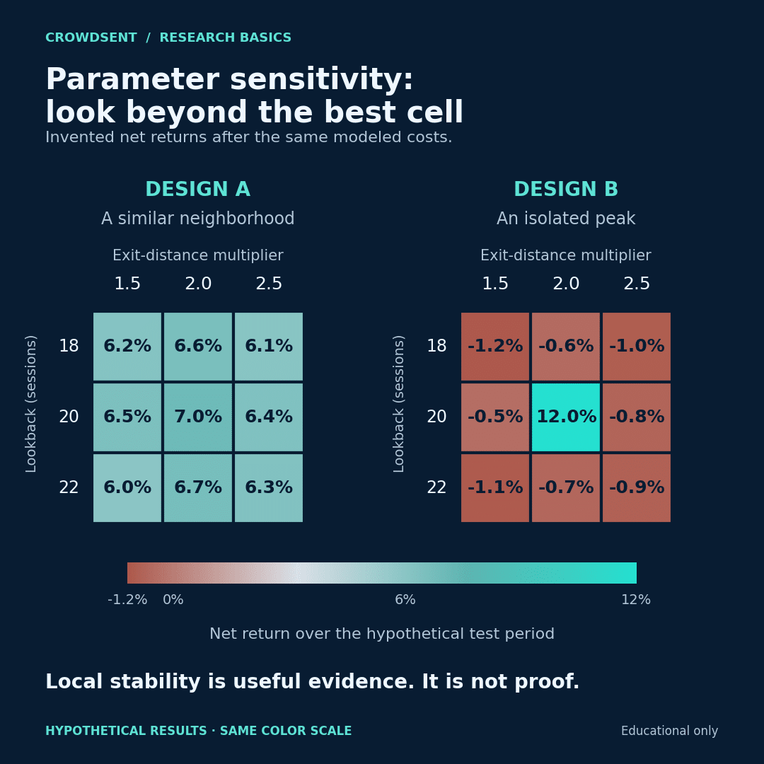
Suppose two fictional rule designs are tested over the same historical development period. Each uses lookbacks of 18, 20 and 22 sessions and exit-distance multipliers of 1.5, 2.0 and 2.5. The following values are invented net percentage returns after the same modeled costs. They are not observed CrowdSent results.
On narrow screens, scroll the table sideways to see every column.
| Lookback | Multiplier 1.5 | Multiplier 2.0 | Multiplier 2.5 |
|---|---|---|---|
| 18 sessions | 6.2% | 6.6% | 6.1% |
| 20 sessions | 6.5% | 7.0% | 6.4% |
| 22 sessions | 6.0% | 6.7% | 6.3% |
On narrow screens, scroll the table sideways to see every column.
| Lookback | Multiplier 1.5 | Multiplier 2.0 | Multiplier 2.5 |
|---|---|---|---|
| 18 sessions | −1.2% | −0.6% | −1.0% |
| 20 sessions | −0.5% | 12.0% | −0.8% |
| 22 sessions | −1.1% | −0.7% | −0.9% |
Design B wins a ranking based only on the largest return. Its neighboring results suggest that the 12% cell needs a detailed decision-level explanation. Perhaps one major trade appears only at that precise setting, or a coding boundary treats one value differently.
Design A shows lower sensitivity within this small grid. That is useful evidence about these settings and this dataset. It does not establish profitability elsewhere, adequate liquidity or a valid information pipeline. A shared error can make every cell look similarly attractive.
The nine cells in either grid are also not nine independent replications. Nearby configurations may execute nearly identical trades. Count them as related research trials and inspect their underlying overlap rather than treating their agreement as nine separate confirmations.
Use more than a return heatmap
For each configuration, retain a compact set of diagnostic measures:
- Loss path: drawdown and the dates of severe losses.
- Participation: number of entries, time exposed and periods with no positions.
- Trading intensity: turnover and modeled transaction costs.
- Concentration: dependence on a few trades, instruments or episodes.
- Implementation: rejected actions, missing inputs and exceptional code paths.
Similar returns can conceal very different behavior. One setting may earn its result through many small moves while another depends on a single large event. Examine trade identities and timing before describing them as equivalent.
A sharp jump also warrants a software check. Verify parameter units, rounding, comparison operators and invalid-value handling. If changing a value from 19 to 20 switches an entirely different branch of the program, the pattern may say more about implementation than economics.
Test interactions and execution assumptions separately
Changing one parameter at a time is easy to interpret, but it can miss interactions. A lookback may appear insensitive when the exit setting stays fixed, yet behave very differently when both move. A small two-dimensional grid can reveal such relationships without launching an unrestricted search.
Then separate parameter changes from scenario changes. For example, repeat the same preselected grid under a clearly labeled higher-cost scenario. This asks whether the apparent neighborhood survives a tougher execution assumption. It does not imply that the stressed cost is a forecast or that the original cost was realistic.
When costs dominate the result, revisit how the bid-ask spread affects a quote comparison. Ensure the cost model matches the type of prices used, so spread or fees are not omitted or accidentally counted twice.
Know what the optimizer actually evaluated
A complete grid evaluates every combination in the specified set. A search algorithm may visit only some combinations. MetaQuotes’ official optimization documentation distinguishes complete enumeration from genetic optimization, which reduces the number of tested combinations.
That matters when drawing a neighborhood. An unvisited cell is unknown, not zero and not evidence of a smooth transition. If the conclusion depends on the immediate neighbors of a selected configuration, run and retain those specific checks rather than interpolating a convincing picture.
Parameter sensitivity should remain a defined diagnostic. Expanding the grid whenever a result disappoints, changing the objective and discarding failed designs increases the amount of selection hidden behind the final chart.
Keep the full selection record
Primary research on the probability of backtest overfitting examines the risk created when historical simulations are used to choose strategies. Sullivan, Timmermann and White’s research on data snooping and trading rules likewise evaluates performance in the context of the rule universe searched.
For a practical research record, save every candidate set, objective, constraint and rerun. Specify a selection rule before opening reserved evaluation data. If that later evidence changes the choice, label the change as another development decision.
Use a market research journal to capture what changed and why. The important claim is narrow: the tested behavior was more or less sensitive to the declared changes under the stated conditions.
Frequently asked questions
1. Is parameter sensitivity the same as optimization?
No. Optimization seeks a configuration according to a selection criterion. Sensitivity analysis examines how behavior changes across specified alternatives. The same runs can inform both activities, but a diagnostic should disclose its range and should not report only the selected winner.
2. Does a broad plateau prove that a strategy is robust?
No. It shows relative stability within the tested neighborhood and assumptions. Shared data leakage, unrealistic costs or exposure to one favorable episode can affect the entire plateau. Additional data, execution checks and independent evaluation still matter.
3. Should I choose the middle of the plateau?
There is no universal rule. A central setting may be a reasonable predeclared selection method, but its meaning depends on the parameter scale and valid range. Explain the choice and evaluate the selected procedure rather than treating geometry as financial evidence.
4. How many neighboring settings should I test?
Enough to answer a specific question about plausible variation and interactions, within the available data and resources. A small, justified grid can be more interpretable than thousands of arbitrary combinations. Record expansions as additional research trials.
5. Why might one parameter change create a large performance jump?
It may change a key trade, cross a discrete threshold or expose a programming issue. Compare the trade lists and relevant code behavior around the boundary. A sharp jump can have a real explanation, but the explanation needs evidence.
6. Can a genetic optimization show every nearby result?
Not necessarily. Search methods can leave combinations untested. Check the actual result list, and evaluate the required neighboring settings explicitly when they support your conclusion. Do not interpret blank cells as poor results or fill them with invented observations.
7. Should I vary position size during the same test?
Only under a clearly specified design. Changing leverage can dominate return and loss comparisons, obscuring the effect of the parameter under study. Preserve the intended sizing policy and explain any mechanical relationship between sizing and other settings.
8. Is a stable Sharpe ratio enough?
No. Also inspect trade count, exposure, drawdown, costs and concentration. The ratio may summarize similar-looking returns while hiding changes in underlying risk or a very small sample. Keep its calculation convention and observation frequency consistent across runs.
9. Can nearby settings be treated as independent evidence?
Usually they are closely related and may share most trades. Their agreement is useful for diagnosing local sensitivity, but it should not be counted as multiple independent demonstrations of an edge. Inspect overlap and avoid overstating sample size.
10. What should I do if every nearby setting performs poorly?
Record the result and revisit the research hypothesis or implementation before widening the search. A negative finding can prevent wasted effort. If you develop a new rule, preserve that change and seek an evaluation that reflects the new version honestly.
Make precision earn its place
To explore the workspace and its membership options, open CrowdSent.
Educational information only, not financial or investment advice. All example returns and configurations are hypothetical. Stable historical results do not guarantee future performance, and trading can result in substantial losses.