

Bond duration vs maturity separates a repayment endpoint from measures built from the whole payment schedule. Maturity tells you when the final scheduled payment occurs. Macaulay duration weights payment times by present value. Modified duration translates that calculation into an approximate sensitivity to a small change in yield.
Those three fields can have different numbers without contradicting one another. The original worksheet below produces a three-year maturity, 2.7355-year Macaulay duration and 2.4869 modified duration from the same fictional bond. Its annual-payment assumptions are chosen for clarity, not to represent a country’s standard bond convention.
Bond duration vs maturity: label the measure first
The FINRA explanation of duration distinguishes maturity from sensitivity and notes that coupon, yield and call features affect the calculation. A field headed only “duration” therefore needs a methodology label before you can reproduce it.
Write three questions beside the fields: When is the last payment scheduled? Where is the present-value-weighted average payment time? How much does the model price change for a small yield movement? Keeping the questions separate prevents a sensitivity statistic from being mistaken for a repayment date.
Start with three explicit payments
Assume face value of 100 currency units, an annual coupon of 10 and exactly three years remaining. The bond is noncallable, its payments are fixed, and valuation occurs immediately after a coupon payment. There is no accrued interest at that point. Ignore default, charges and taxes within this mathematical exercise.
The remaining payments are 10 after one year, 10 after two years, and 110 after three years. The final 110 combines the last coupon with 100 of principal. Use an annual yield of 10%, written as 0.10, and annual compounding throughout.
For each row, divide its payment by 1.10 raised to the number of years until payment. The first present value is 10 ÷ 1.10 = 9.090909. The second is 10 ÷ 1.10² = 8.264463. The last is 110 ÷ 1.10³ = 82.644628.
On a narrow screen, scroll the table sideways to read every column.
| Year | Payment | Present value | Year × present value |
|---|---|---|---|
| 1 | 10 | 9.090909 | 9.090909 |
| 2 | 10 | 8.264463 | 16.528926 |
| 3 | 110 | 82.644628 | 247.933884 |
| Total | 130 | 100.000000 | 273.553719 |
The model price is the sum of the present values: 100. The undiscounted 130 belongs in a separate total. Dividing the weighted column by 130 would mix discounted and undiscounted quantities and would not reproduce the measure we are calculating.
For a simple worksheet test, double every payment and the face amount. Present values and model price double, while the relative weights stay unchanged. A duration result that doubles under this test probably contains a missing division by price.
Turn the present values into duration
The Reserve Bank of India’s securities primer, section 27, describes the present-value weighting and the adjustment to modified duration. We apply those concepts to the independent annual-pay example here, rather than copying the primer’s semiannual illustration.
Divide each row’s present value by 100 to obtain its weight. The weights are approximately 9.0909%, 8.2645% and 82.6446%, summing to 100%. Most of the present value belongs to the third payment, so the weighted time sits relatively close to year three.
Macaulay duration = sum of time × present value ÷ model price. Here, 273.553719 ÷ 100 gives 2.735537 years. This weighted average is earlier than the final payment because the first two rows carry positive weight. It does not create a new payment at year 2.735537.
For this annual-compounding model, divide Macaulay duration by one plus the annual yield: 2.735537 ÷ 1.10 = 2.486852. This is the modified duration. With a yield quoted at m compounding periods per year, the corresponding adjustment uses 1 + yield/m and a consistently expressed Macaulay duration.
Keep full calculation precision behind the display. If you first round Macaulay duration to 2.74 and then divide, the modified result becomes approximately 2.4909. That small difference is avoidable and can confuse a later comparison against independently recalculated prices.
Compare the duration estimate with exact repricing
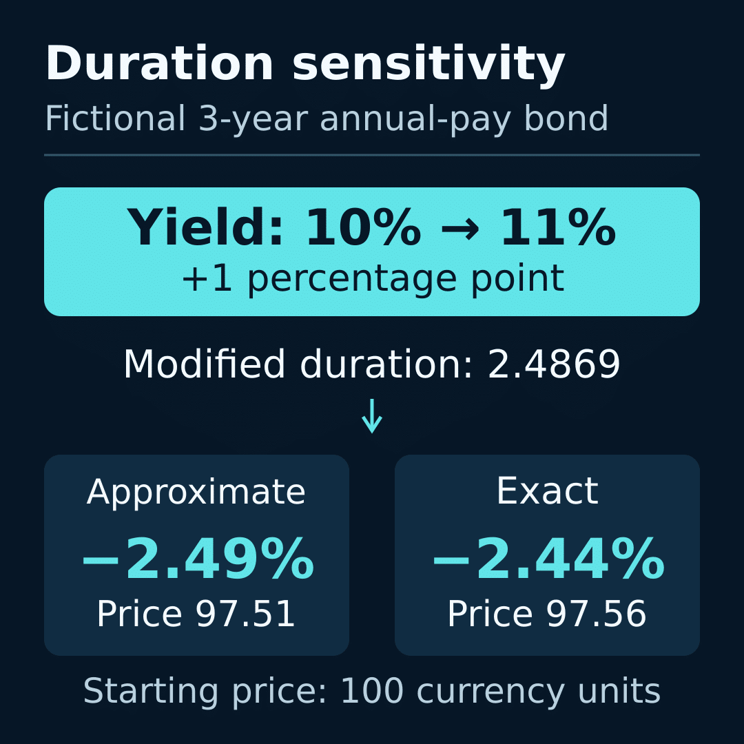
Raise the hypothetical yield from 10% to 11% while keeping the three payments and their times fixed. This changes the decimal yield by 0.01. The first-order relationship is approximate proportional price change = −modified duration × yield change.
Our estimate is −2.486852 × 0.01 = −0.02486852, or −2.486852%. Applied to the starting price of 100, it gives 97.513148. The negative sign follows from this model’s response to the specified upward yield change; it is not a prediction that yields will rise.
Now recalculate each payment using 1.11: 10 ÷ 1.11 + 10 ÷ 1.11² + 110 ÷ 1.11³ = 97.556285. Exact repricing within the stated model gives a −2.443715% change. The two prices differ by 0.043137 currency unit per 100 face.
The duration estimate is a local straight-line approximation to a curved price relationship. The discrepancy remains even when every arithmetic step is correct. To see its size change, repeat with a smaller yield move to 10.50%: the approximation gives 98.756574, exact repricing gives 98.767438, and the gap is about 0.010864.
“Exact” here means exact for the specified cash flows and discounting formula. It does not certify an executable market price. A real quote needs its own timestamp and bid or ask label, and may reflect assumptions outside this exercise.
Keep the assumptions attached to the number
Store the valuation date, remaining payments, time units, yield convention, duration type and price basis together. A field with a different method label needs its own documentation. If payments can change, our fixed three-row schedule may no longer describe the scenario being measured.
Use the market research journal template to preserve the inputs and both repricing results. When checking a published figure, trace it to the original methodology before trying to make your spreadsheet match it.
FINRA also cautions that low duration does not remove other bond risks. This worksheet isolates one price-sensitivity calculation. It supplies no evidence about payment reliability, inflation, currency changes or the terms available for a transaction.
Frequently asked questions
Can two bonds have the same maturity and different durations?
Yes. Moving payment weight into earlier years changes the weighted average even if the last payment stays in year three. To compare two records, inspect their full schedules and discounting assumptions rather than using the maturity field as a substitute.
Does Macaulay duration identify a guaranteed payback date?
No payment occurs at 2.735537 years in this example. Payments occur at years one, two and three. The duration result is an average constructed from their present values; it should not be added to the calendar as a promised cash-recovery event.
Why are Macaulay and modified duration different?
They answer different worksheet questions. Macaulay duration weights payment times; modified duration adjusts that result for the yield convention to express local price sensitivity. In our annual-pay example, dividing 2.735537 by 1.10 gives 2.486852.
Why does the 10% to 11% change enter as 0.01?
The formula uses decimal yields: 0.11 minus 0.10 equals 0.01. Inserting 1 would make the modeled shock one hundred times larger. Write both the percentage-point change and its decimal equivalent beside the calculation to expose unit errors.
Is the duration estimate an exact price forecast?
It is an approximation under a specified shock. Our 97.513148 estimate differs from the directly recalculated 97.556285 even though both use identical payments. Neither number establishes where a future market transaction will occur.
What does convexity explain in the example?
It describes the curvature omitted by the first-order estimate. At an 11% yield, exact model price exceeds the duration estimate by about 0.043137. The smaller shock to 10.50% produces a smaller gap, making the approximation’s local nature visible.
When would Macaulay duration equal maturity?
In a fixed-payment example with only one remaining positive cash flow, all present-value weight sits at that payment’s time. A single payment three years away therefore has three-year Macaulay duration. Its modified duration still requires the yield-convention adjustment.
Can a bond fund report duration without one maturity date?
A collection of positions can have an aggregate sensitivity statistic while its constituent payments occur on many dates. Check what the fund’s reported statistic measures. It should not be interpreted as a single date on which every holding repays principal.
Why do callable or floating-rate bonds need additional care?
Our exercise keeps payment amounts and timing fixed under the yield shock. A model allowing either to change needs additional assumptions. Read the documented method for that instrument or duration field before reusing this three-payment formula.
Does a smaller duration establish lower overall risk?
It establishes no such conclusion by itself. The worksheet varies a yield input and observes modeled price sensitivity. It does not test whether payments occur, whether purchasing power changes or whether a position can be sold on acceptable terms.
Educational explanation by the CrowdSent Blog Team. Sources checked 13 October 2026. All worked figures are hypothetical and are not investment recommendations.