

By CrowdSent Blog Team
A Bollinger Bands calculation combines a moving average with the standard deviation of a selected price series. In the traditional form, the middle band is a simple moving average, and the upper and lower bands sit a chosen number of standard deviations above and below it. The result is a changing reference envelope around recent prices.
Reading that envelope accurately requires more than spotting a touch of the upper or lower line. You need to know which prices entered the calculation, how dispersion was measured, and whether the observation was complete. This guide builds a small example from scratch and separates three questions: where the center is, how wide the bands are, and where the close sits within them.
This educational explanation uses hypothetical data and does not recommend trades.
What goes into the Bollinger Bands calculation?
For a chosen window of n observations, calculate the middle band as their arithmetic mean. Calculate standard deviation over that same window. Then add k times the standard deviation to obtain the upper band, and subtract k times it to obtain the lower band. The multiplier k controls the distance of each outer line from the center.
Written compactly: middle = mean; upper = mean + k × standard deviation; lower = mean − k × standard deviation. MetaTrader’s Bollinger Bands reference gives this construction and a standard-deviation formula that divides squared deviations by n.
The familiar setting of 20 periods and two standard deviations is a default convention. It is not a mathematical requirement that all markets use twenty daily closes. A period can be an hourly bar, a daily session or another defined interval, and chart settings may offer a price source other than close.
State the standard-deviation convention
For the version used here, subtract the window’s mean from each price, square each difference, add those squares, divide by n, and take the square root. A spreadsheet’s sample standard deviation instead divides by n − 1. Those choices produce different answers, especially in short demonstration windows.
A calculation sheet should therefore name the convention rather than merely label a cell “SD.” This is a reproducibility issue. A wider band caused by choosing the sample formula is not evidence that the underlying prices became more volatile.
A five-price worked example
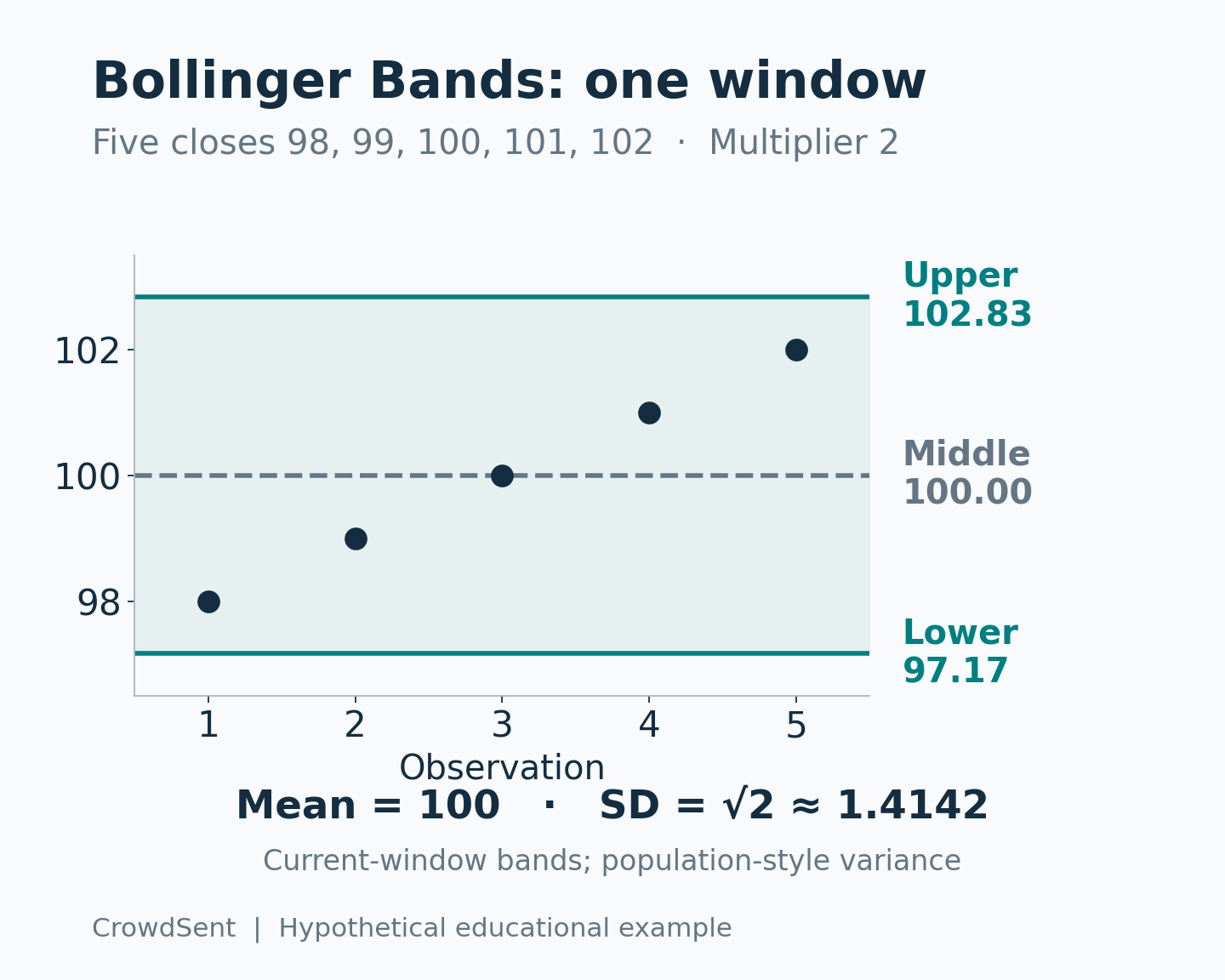
Use five hypothetical closing prices: 98, 99, 100, 101 and 102. Five observations keep the arithmetic short; they are not a proposed indicator setting. The total is 500, so the mean is 500 ÷ 5 = 100. Each price differs from the mean by −2, −1, 0, 1 or 2.
Squaring these deviations gives 4, 1, 0, 1 and 4. Their sum is 10. Dividing by five gives variance 2, and taking the square root gives standard deviation approximately 1.4142. With a multiplier of two, the distance from the middle band to either outer band is approximately 2.8284.
The upper band is therefore 102.8284, the middle band is 100, and the lower band is 97.1716. The latest close of 102 lies inside the envelope, nearer the upper edge. Nothing in this arithmetic tells us the next closing price.
Now compare the sample formula
If the same squared deviations were divided by four instead, variance would be 2.5 and standard deviation approximately 1.5811. The resulting bands would be approximately 103.1623 and 96.8377. The observations, window length and multiplier have not changed. Only the variance convention has.
This controlled comparison is useful when a worksheet disagrees with a platform. First verify the five inputs, then the mean, then the standard deviation. Changing multiple settings together makes the source of a discrepancy harder to identify.
What happens when the window moves?
Add a new hypothetical close of 104 and remove the oldest close, 98. The new window is 99, 100, 101, 102 and 104. Its mean is 101.2. The squared deviations are 4.84, 1.44, 0.04, 0.64 and 7.84, totaling 14.8. Variance is 2.96 and standard deviation is approximately 1.7205.
At the same multiplier of two, the updated outer bands are approximately 104.6409 and 97.7591. The center moved up, and the band distance increased. Keeping those two changes separate makes the chart easier to explain: both location and dispersion changed, for different arithmetic reasons.
Change the multiplier while holding the prices fixed
Keep the original five closes, their mean of 100 and their standard deviation of approximately 1.4142. Change only the multiplier from two to one. The new upper band is 101.4142 and the lower band is 98.5858. Their total width is approximately 2.8284, half the earlier 5.6569.
The latest close is still 102. It now lies above the upper band, although it was inside the two-standard-deviation envelope. Neither the price observations nor their measured dispersion changed. A chart label switched because the envelope setting changed.
The corresponding %b ratio becomes approximately (102 − 98.5858) ÷ 2.8284 = 1.2071, compared with 0.8536 under the original setting. Keep full precision until the final rounding step. This controlled comparison shows why a band touch or an out-of-band reading must travel with its multiplier. Recomputing the mean is unnecessary when the data window and source prices remain identical.
BandWidth and %b answer different questions
A raw band width is simply upper minus lower. In the initial example, it is approximately 5.6569 price units. To express the width relative to the center, one common percentage convention is BandWidth = 100 × (upper − lower) ÷ middle. With a middle band of 100, that equals approximately 5.6569%.
Always check display units. A platform showing the ratio without multiplying by 100 would display about 0.056569 for the same example. That is a scaling difference, not a hundredfold disagreement about the market.
The %b measure describes location within the envelope: %b = (close − lower) ÷ (upper − lower). At a close of 102, %b is approximately (102 − 97.1716) ÷ 5.6569 = 0.8536. On this ratio scale, zero corresponds to the lower band, 0.5 to the middle and one to the upper band.
A value above one means the selected price is above the upper band. A value below zero means it is below the lower band. The name can be confusing because some displays scale the ratio into percentage points. Record the formula or scale next to the reading.
John Bollinger’s own rules distinguish relative price location from band width and emphasize that touching a band alone is not a transaction signal. A relatively high price within an envelope is a description of its position, not a valuation judgment about the asset.
What narrowing or widening bands can establish
For an unchanged multiplier and calculation method, a smaller raw band width means a smaller standard deviation in the selected price window. A larger width means a larger one. That is the direct mathematical conclusion. Any claim about when a future move will happen, or which direction it will take, requires more than this identity.
For example, compare two invented windows centered at 100. In one, standard deviation is 1; in the other, it is 3. With multiplier two, their total widths are 4 and 12. This says the second window’s prices were more dispersed around its mean. It does not say that tomorrow’s range will be three times larger.
Be especially careful with the phrase “95% of prices.” Two standard deviations are familiar from particular probability models, but drawing bands does not establish that those models fit a security’s prices. Bollinger explicitly cautions against importing statistical assumptions just because standard deviation appears in the construction.
A changing envelope is not a fixed boundary
The outer lines move when the input window changes. A price can remain near one edge across several bars while the center and edges shift. It is therefore misleading to describe an upper-band touch as reaching a permanent ceiling. Fidelity’s indicator guide describes the bands as standard-deviation envelopes around an average.
Historical news can help explain why the underlying observations changed, but attaching a story after looking at a chart is easy. Verify the event’s timing and source before making a causal claim. CrowdSent’s guide to verifying market news provides a separate evidence check.
A practical reconciliation checklist
When two charts show different bands, compare their instrument, venue, session, time zone, bar duration, source field, adjustment policy, window length, multiplier, averaging method and standard-deviation convention. Confirm that neither chart uses a displaced overlay whose lines are plotted against a shifted timestamp.
A live final bar also deserves a label. If its current price is being treated as its provisional close, the average and dispersion may change before the bar ends. An earlier screenshot and a completed-bar export can disagree without either record being corrupted.
Do not repair missing observations by inserting zero prices. A fabricated zero can pull the center down and greatly widen the envelope. The distinction between missing market data and zero matters before any comparison of bands.
Save a small audit record with the source, exact settings, completed-bar status and a few sample calculations. A market research journal is useful for keeping these definitions beside the interpretation, so a later reader can identify which part was measured and which part was inferred.
Frequently asked questions about Bollinger Bands
1. What do the three Bollinger Bands lines represent?
The middle line represents the chosen average. The outer lines add and subtract a dispersion-based distance from that center. Their roles are easiest to understand separately: center describes average location, outer distance describes spread around that location.
2. Must Bollinger Bands use a twenty-day window?
No. Twenty is a common period count, and the bar duration is a separate choice. Twenty hourly observations are different from twenty daily observations. A meaningful comparison names both the count and the duration instead of assuming every period is a day.
3. Why might my spreadsheet produce wider bands?
One possible cause is using sample rather than population-style standard deviation. Different source prices, session boundaries or multipliers can also explain it. Reconcile the mean and variance in order before changing the chart settings to force a match.
4. Does touching the upper band mean an asset is expensive?
It means the selected price is relatively high within this particular envelope. It does not establish intrinsic value or affordability. A valuation conclusion would require a different question and appropriate financial evidence beyond the recent price distribution.
5. Does a squeeze predict a specific breakout direction?
Narrow bands describe reduced dispersion under the chosen settings. Their width alone does not encode an upward or downward direction for the next move. Nor does a narrow reading provide a deadline by which a large move must occur.
6. Are prices guaranteed to stay inside the bands?
No. The outer lines are calculated references, and prices can lie beyond them. Treating the envelope as a guaranteed interval would add an assumption that the calculation itself does not justify, especially when the same current price helps determine its boundaries.
7. What is the difference between BandWidth and %b?
BandWidth describes the distance between the outer lines, often normalized by the middle line. The %b ratio describes a selected price’s position between those lines. One can change without the other moving in the same direction.
8. Can %b be above one or below zero?
Yes. On the ratio scale, an above-upper-band price gives a value above one, and a below-lower-band price gives a negative value. If a display uses a percentage scale, the equivalent reference levels are 100 and zero.
9. What happens when every price in the window is identical?
Standard deviation is zero and the bands coincide. The %b denominator then becomes zero, so the ordinary formula is undefined. A platform may leave a gap or apply a special convention; a worksheet should flag the case rather than divide blindly.
10. Can two assets have the same BandWidth but different prices?
Yes, when BandWidth is normalized. For example, a width of 4 around a middle value of 100 and a width of 20 around 500 both equal 4%. Comparable ratios still require comparable windows, price sources and calculation settings.
Conclusion: separate center, spread and location
A careful Bollinger Bands calculation makes three distinct quantities visible: the average, the dispersion around it, and the selected price’s place within the resulting envelope. Work through those quantities before applying labels such as wide, narrow, high or low. Clear inputs and an explicit variance convention make the result reproducible; they do not turn the envelope into a forecast.
Source documentation checked 11 October 2026. Educational explanation from the CrowdSent Blog Team. Numerical examples are hypothetical unless explicitly identified otherwise. This article does not provide investment recommendations.